Program "XY-Function"
Graphical representation and interpolation of XY functions given on unstructured grids of XY-points
Copyright: Helm Ing. 1999-2000
- Short Description of the Program
- Delaunay Triangulation
- Program Structure
- File Format
- Grid to Grid Interpolation
- Short Tutorial
- XY-Function enables 2D and 3D presentations of data given
on unstructured grids of XY-points.
- The mathematical approach is based on the DELAUNAY triangulation.
- For this test version the number of points is restricted to 2000.
- The values and XY-coordinates can be read or saved with text files or
they can manually be added one by one.
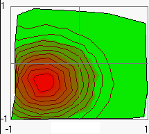
- 2D-Images with arbitrary numbers of contour
lines and arbitrary colors can be generated.
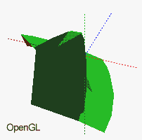
- 3D-images (by using OpenGL) of functions can be drawn and
rotated to get a better spatial impression of the data.
- Interpolated values of the function belonging to arbitrary coordinates are displayed simultaneously with the mouse movement.
- Interpolations of a complete function belonging to other, arbitrary grids of points are supported.
- XY-Function requires OpenGL 1.1 (contained in Win 98/ME/NT) to present 3D-images.
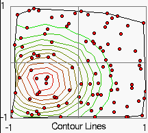
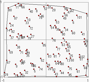
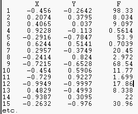
Values will be given (or measured) often on points which are randomly distributed in two dimensions:
Here a function was determined at 102 points given within the range: -1 < x,y < 1.
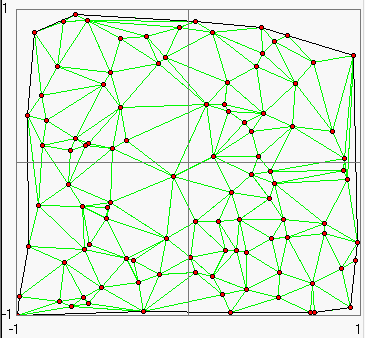
To represent this data as a continuous function the XY-plane may be divided into triangles by using the DELAUNAY triangulation:
The following conditions should be fulfilled at this:
- The variation in the area of the triangles should not be too large.
- The aspect ratio of triangles should be as close to 1 as possible.
The aspect ratio is defined as the ratio of the circumradius of the triangle to twice its inradius. Hence the aspect ratio of an equilateral triangle is exactly 1.
- The ratio of the largest to the smallest edge/angle of each triangle should be close to 1.
- The ratio of the area of the largest/smallest triangle to all the immediate neighbours should not be drastically low/high.
Calculations of contour lines can be executed for each triangle one by one. This requires only linear interpolations.:
The triangulation is also usefull for applications of OpenGL or Direct3D which can calculate 3D presentations of 2D-functions based on meshes of triangles.
The XY-Function main form comprises the following fields:
- Load a function as text file (cfg. File Format, for example load file1.txt),
- Save the function as text file,
- Delete all XY-points and the corresponding values,
- Copy the actual picture to clipboard,
- Grid to grid interpolation,
- Example: Generates random points of a GAUSS distribution as long as the button is pressed,
- Open this help file.
2. Mode Register
It consists of two sheets:
2D (Contour Lines)
- 2D-Parameter Register
- XY-Range:
The edit fields are used for setting the default XY-range of the 2D-Image.
- Show:
With the check boxes You can switch on the drawing of points, trajectory etc. or the elements of designation (numeration of points, iso colors...). Be carefully with the coloration mode, it works slow!
- IsoColors:
The number of contour lines and the colors of the maximum and minimum line can be choosen here. For color change click on the corresponding field.
- Design:
Here you can change the used font and the title of the 2D-Image. Furthermore the number of auxiliary lines may be set here.
- Regular Grid:
A regular grid can be generated with arbitrary x- and y-steps with respect to the actual default range. The grid may be saved and can be used as a target grid for a grid to grid interpolation (button 5).
- Data Table
The table shows the numbered XY-coordinates and function values which can not be edited in this test version of the program. By marking the check boxes Points and Numbers on the Show sheet all numbered points will be drawn into the 2D-Image.
- 2D Image Field
The visible range of the function may be enlarged and scaled-down (zoomed) by mouse dragging (with the left mouse button) from above on the left to down on the right. Inverse mouse dragging from down on the right to above on the left restores the default XY-range.
The values and XY-coordinates can be added manually one by one with a click of the right mouse button on the corresponding position of the 2D-image field.
3D (OpenGL)
The distance to the 3D-Image of the function may be changed with the trackbar Focal Length. Furthermore the the 3D-Image can be rotated by mouse dragging (tilting of the Z-Axis) or changing the trackbar Turn around Z. The coordinate axis X,Y and Z may be displayed marking the check box Show Axis.
3. Status Bar
2D: XY-coordinates and the interpolated values on the mouse position in the 2D-image,
3D: direction of the Z-axis and the turn angle about the Z-axis.
For each data point one line must be filled with three values for X,Y and F:
For the input file for the Grid to Grid Interpolation only two values for X and Y are necessary for each line.
Before pressing the corresponding tool button 5 You have to prepare a file in which the new set of points is described (two numbers for each line, cfg. file format). These points should be within the convex hull of the point set of the starting (current) function.
Values of points near but outside the convex hull will be roughly estimated only.
After loading this file the current function will be interpolated to the new set of points.
The result is decribed in a message box:
... points were read in,
... values were interpolated correctly,
... values were estimated roughly,
... values could not be estimated.
The interpolated values will be inserted in the grid file:
1. Loading a function
There are four examples named file1.txt ... file4.txt, you can load and view. Before loading a new file You should delete the old data by pressing the Delete button 3.
2. Changing 3D-Parameters
- Load an example file and set the mode register on 3D (OpenGL),
- Testing the effect of setting the Focal Length, Turn around Z and Show Axis elements,
- Rotate the 3D-Image by tilting the Z-Axis (mouse dragg).
3. Changing 2D-Parameters
- Load an example file and set the mode register on 2D (Contour Lines),
- Testing the effect of setting the parameter registers XY-Range, Show, Iso-Colors and Design,
- The visible range of the function may be zoomed by mouse dragging (with the left mouse button) from above on the left to down on the right. Inverse mouse dragging from down on the right to above on the left restores the choosen XY-Range.
4. Manual addition of data
- Set mode register on 2D (Contour Lines),
- Choose a initial file or press the Delete button 3 to generate a new data set.
- Add a new data point with a click of the right mouse button on the corresponding position of the 2D-Image field.
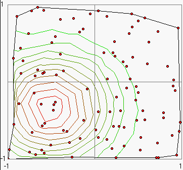
5. Example: Random points of a GAUSS function
As long as the Example button 6 is pressed random points of a GAUSS function at x = -0.5 and y = -0.33 will be generated.
If the mouse points to the centre of the distribution presented in the 2D-Image, You can read out the maximum parameter from the status bar .
6. Generation of a reguar grid
Set the 2D-Parameter register on Regular Grid.
A regular grid with arbitrary X- and Y-steps (with respect to the actual default range) can be generated and saved. The actual data set will be deleted at this.
7. Grid to Grid Interpolation
- Generate a XY-function by pressing the Example button 6 for a short time,
- Save this function Save button 2,
- Generate and save a regular grid of points with X steps= 10,Y steps= 10 (i.e. 11 * 11 points, ) - the XY-range should be unchanged at this,
- Reload the function and press the Interpolation button 5,
- Choose the generated grid, the corresponding file will be modified as described above (cfg. Grid to Grid Interpolation).